Skip to content
recaplica

    One moment: security check

    Cloudflare wants to make sure you're not a robot. Tick the box below and your search will continue on its own.

    IT
    recaplica Probability and Statistics: What They Are and How They Work Together
    © 2026 Recaplica · recaplica.com — All rights reserved
    Home › Science

    Probability and Statistics: What They Are and How They Work Together

    By Recaplica Newsroom · Updated on September 18, 2026

    What to print

    Page numbers appear when printing with default margins.

    Slides

    Choose a cut

    Flash10 slidesThe essential thread, to present in classFull15 slidesEvery chapter and the deeper detail

    Both come with speaker notes.

    Telegram channel
    recaplica Clear in 30 seconds, yours in 10 minutes.
    In 30 seconds Key points Figures Deep dive Slides Myths Mind map Quiz Flashcards FAQ

    In 30 seconds quick read

    Probability and statistics are two branches of mathematics that study uncertainty from opposite directions: probability calculates ahead of time how likely an event is to happen, while statistics analyzes data already collected, either to describe it or to draw conclusions about a wider group. Introductory math courses teach them together because they share the same basic tools, from the idea of an event to that of a sample. Statistics itself splits into descriptive statistics, which summarizes data with numbers like the mean and standard deviation, and inferential statistics, which uses a sample to estimate an entire population. Probability, in turn, is calculated differently depending on whether outcomes are equally likely (classical probability, like a die roll) or observed over time (frequentist probability, like equipment failures).

    Key Points

    • Probability and statistics are two branches of mathematics that study uncertainty: one deals with events that haven't happened yet and how likely they are, the other with data already in hand, summarized or used to draw conclusions.
    • Descriptive statistics summarizes data with numbers such as the mean, median, and mode; inferential statistics uses a sample to draw conclusions about a larger population.
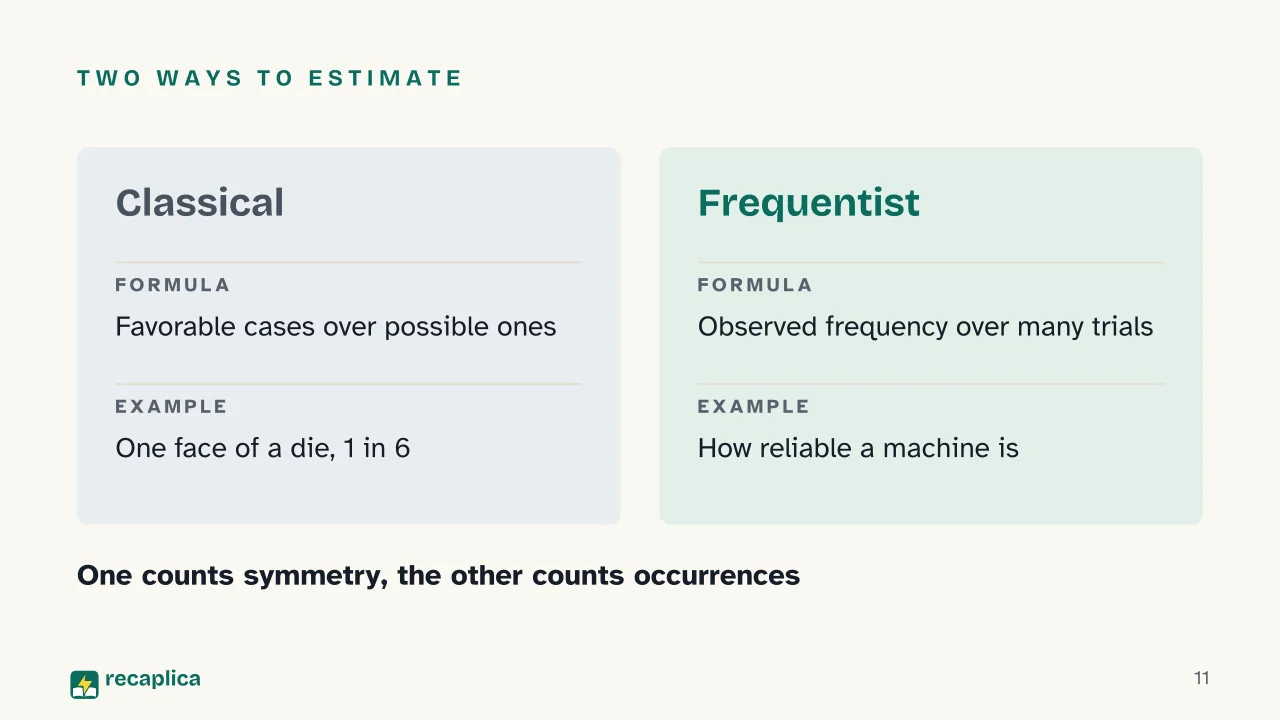
    • Classical probability divides favorable outcomes by possible outcomes, as with a die roll; frequentist probability is estimated by observing how often an event occurs across many trials.
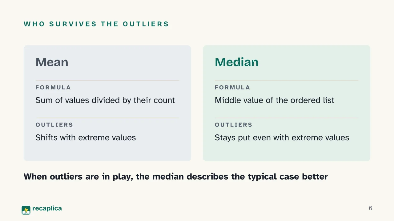
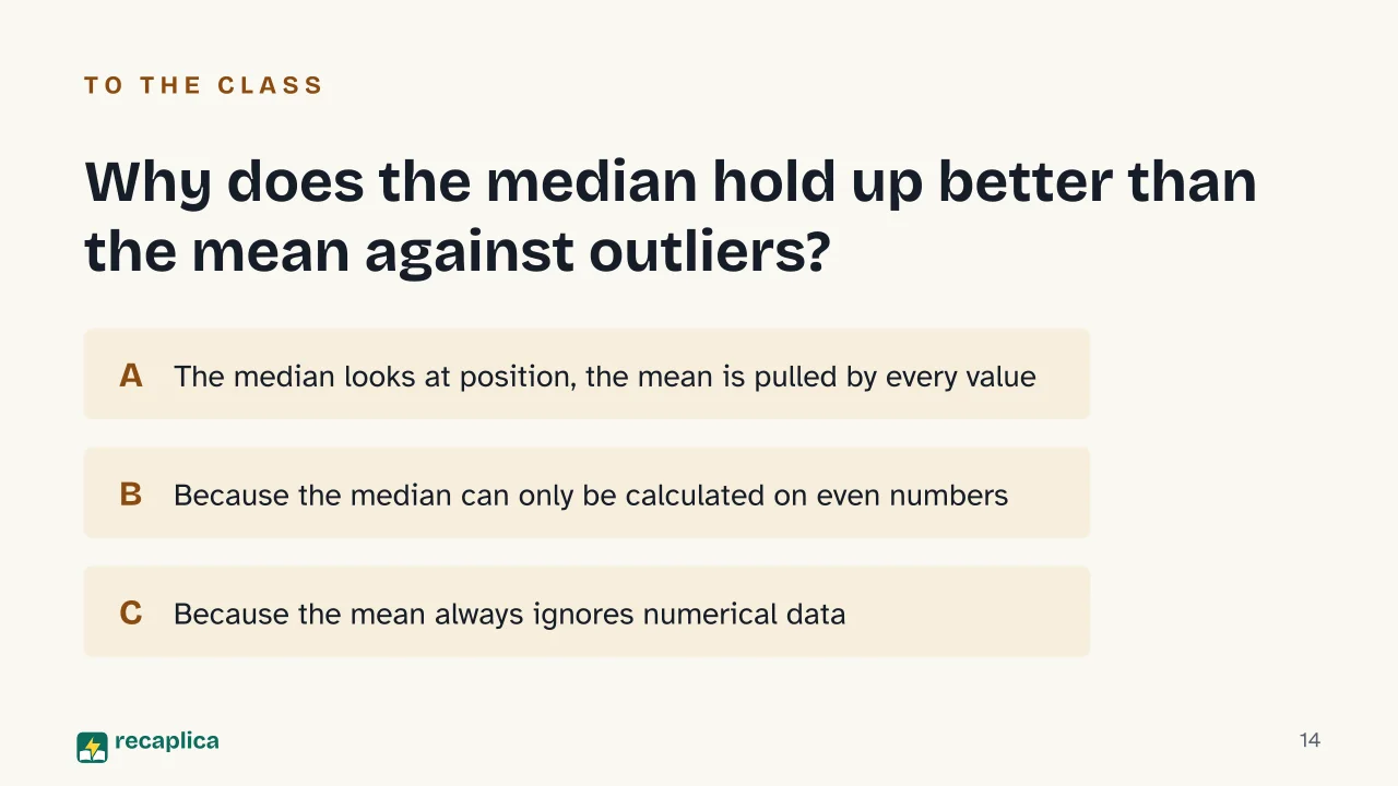
    • The mean is the sum of all values divided by how many there are, and it shifts with extreme values, while the median, the middle value of an ordered list, stays stable even when the data includes outliers.
    • Standard deviation measures how far data points typically sit from the mean: small when values cluster together, large when they're spread out.
    • Coin flips are independent events: each flip has a 1/2 probability, no matter what came before it.

    Key figures

    • 58,943,673 Residents counted in Italy, a recurring census figure that is itself a plain example of descriptive statistics applied to a real population. Source: ISTAT (Italian National Institute of Statistics), Resident population, as of June 30, 2026

    Deep Dive

    Probability and statistics are two subjects that, in introductory high school math courses, almost always travel together, even though they look at uncertainty from opposite directions. As OpenStax puts it, statistics deals with the collection, analysis, interpretation, and presentation of data; probability, on the other hand, is the mathematical tool used to study randomness, meaning how likely an event is to happen. Someone rolling a die uses probability to predict; someone who has already logged a thousand rolls uses statistics to describe what actually happened.

    Descriptive statistics and inferential statistics

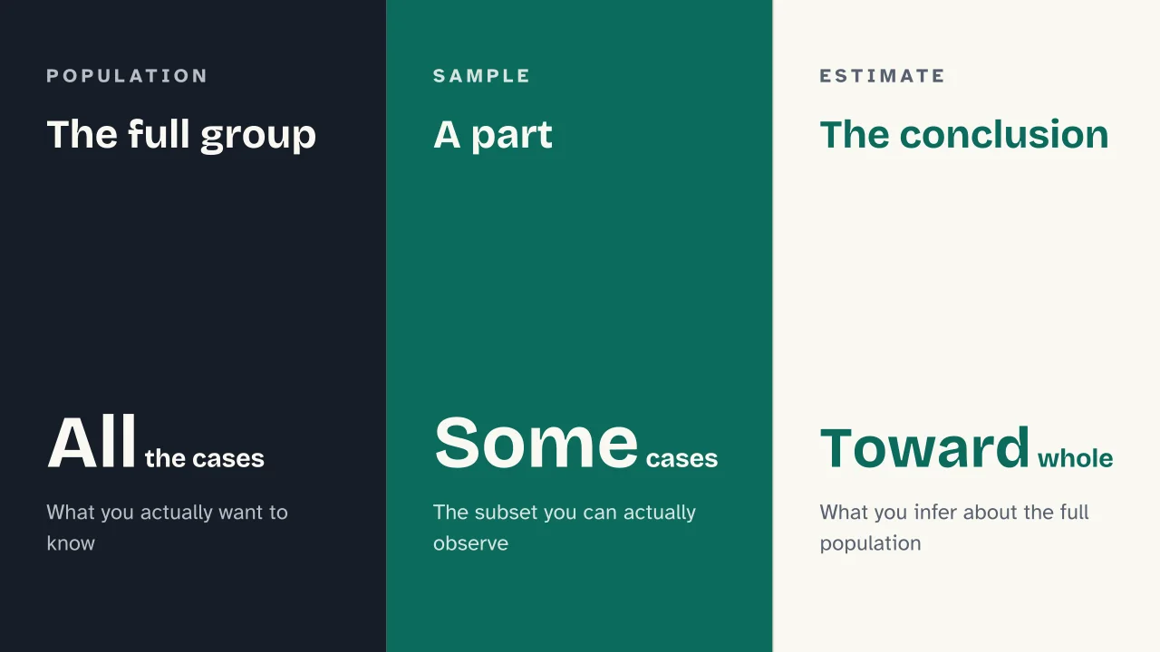
    Statistics splits into two branches. Descriptive statistics organizes and summarizes data that has already been collected: it counts, sorts, and calculates averages. Inferential statistics, according to OpenStax, is the set of formal methods for drawing conclusions from “good” data (collected with sound criteria), and it comes into play when observing an entire group isn’t possible. That requires two key concepts: the population, meaning the collection of people, things, or objects under study, and the sample, a portion of that population selected to gather information from. A value calculated over the whole population is called a parameter; the same kind of value calculated over a sample is called a sample statistic, used to estimate the corresponding parameter.

    AspectDescriptive statisticsInferential statistics
    What it doesSummarizes the data on handEstimates characteristics of a population
    What it works onThe entire set of collected dataA sample, a portion of the population
    Typical toolsMean, median, mode, standard deviationEstimates, intervals, tests on a sample
    ExampleA national statistics office counts residentsA survey of a thousand people estimates a national opinion

    A clean example of descriptive statistics on its own is a population count: according to ISTAT, Italy’s national statistics institute, the resident population stood at 58,943,673 as of June 30, 2026. That’s not an estimate drawn from a sample: it’s a count, updated periodically, of the entire population — the simplest case of descriptive statistics applied to a real number.

    The measures that summarize a group of numbers

    To summarize a set of numbers, descriptive statistics relies on three measures of central tendency. The mean is the sum of all values divided by how many there are, the same addition-and-division operation covered in Arithmetic, just applied to a whole group of numbers instead of two. The median is the value sitting at the center of an ordered list: at least half the data is less than or equal to it, and at least half is greater than or equal to it. The mode, more simply, is the value that shows up most often in the set.

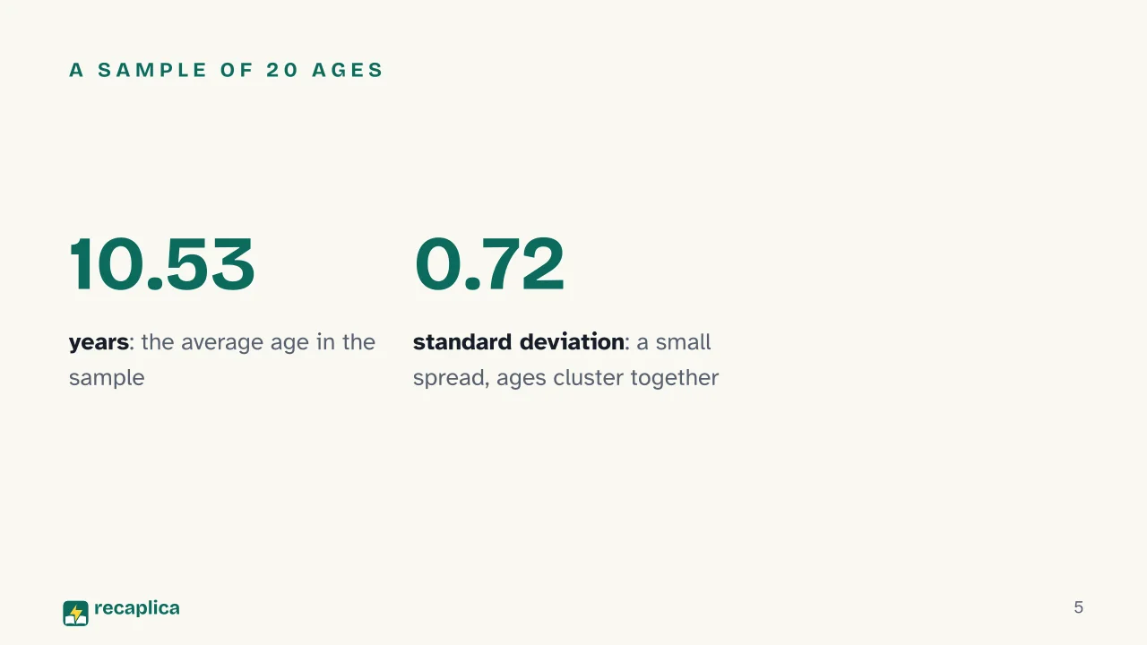
    Worked example: OpenStax lists the ages of 20 students in a fifth-grade class: 9, 9.5, 9.5, 10, 10, 10, 10, 10.5, 10.5, 10.5, 10.5, 11, 11, 11, 11, 11, 11, 11.5, 11.5, 11.5. Adding up all the ages and dividing by 20 gives a mean of 10.53 years. Sorted, the middle value (the median) falls right inside the “10.5” cluster, very close to the mean — a sign that in this case the data is fairly symmetric, with no outliers pulling the mean off to one side.

    When a set instead contains values much higher or lower than the rest, the mean and median start to drift apart. OpenStax ties this directly to the shape of the distribution: the mean is affected by outliers that don’t influence the median, so in a left-skewed distribution the mean tends to sit below the median, and in a right-skewed one it tends to sit above it. That’s why, when a single number has to describe a very uneven group, the median is often the more honest choice.

    How spread out is the data: standard deviation

    Knowing only the mean of a group isn’t enough: two classrooms can share the same average age with very different makeups, one where every age is close together, another mixing much younger and much older kids. Standard deviation is the number that captures exactly this: how far, on average, the values in a set sit from their own mean. It’s small when the data clusters near the mean, larger when the values are spread out.

    In the 20-age example, the sample standard deviation OpenStax calculates is 0.72: a low figure, consistent with a group of children who are nearly all the same age. The formula uses the same letters and symbols found in expressions from Algebra: s = √[Σ(x − x̄)² / (n−1)], where x̄ is the mean and n is the number of values. One technical detail explains why the differences from the mean get squared instead of simply added up as they are: adding the deviations from the mean without squaring them always produces zero, because the positive and negative gaps cancel each other out.

    Classical probability and frequentist probability

    Probability, too, can be calculated in more than one way. According to the Stanford Encyclopedia of Philosophy, the classical interpretation defines the probability of an event as the fraction between the number of cases in which the event occurs and the total number of possible cases — a formulation that traces back to the mathematician Abraham de Moivre, who described it as the fraction with, in the numerator, the number of ways an event can happen, and in the denominator, the total number of ways it can either happen or fail.

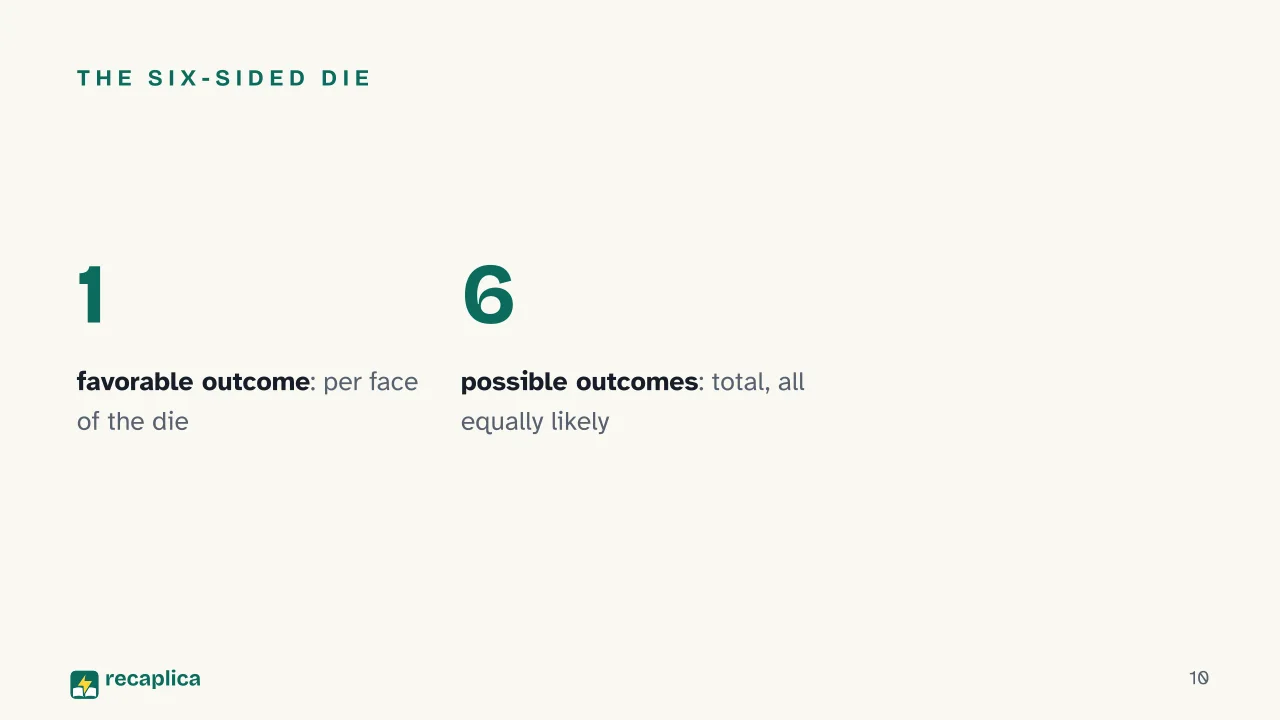
    Worked example: a six-sided die has six possible outcomes, all equally likely by the symmetry of the object; the set of these outcomes is called the sample space. The classical probability of rolling a 4 is therefore 1 favorable case out of 6 possible cases, or 1/6. The same logic applies to a coin: two possible outcomes, heads or tails, each with a probability of 1/2.

    Classical probability works well when outcomes are equally likely by construction, like the faces of a fair die. But many real-world events don’t come with that kind of built-in symmetry: how many times a machine breaks down in a year can’t be worked out by dividing favorable cases by possible cases. That’s where frequentist probability comes in, defined by the Stanford Encyclopedia of Philosophy as the relative frequency with which an attribute actually shows up within a reference class: the event is observed many times, and the proportion of times it occurred is calculated. Further along in a math curriculum, once these observed frequencies turn into continuous distributions studied through functions and limits, the territory becomes calculus.

    Independent events and the gambler’s fallacy

    Two events are called independent when one occurring doesn’t change the probability that the other occurs. Statistics LibreTexts defines independence this way, and this exact property is what dismantles one of the most common mistakes tied to games of chance.

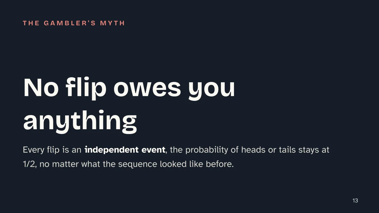
    Worked example: after five coin flips in a row that all came up heads, many people think that on the sixth flip tails is somehow “more likely,” as if the coin needed to balance out the sequence. Statistics LibreTexts calls this reasoning the gambler’s fallacy: people who fall for it imagine a natural adjustment compensating a run of heads with more tails later on. But the coin carries no memory of the flips before it: on the sixth flip, the probability of heads is still 1/2, exactly as it was on the first.

    There’s one related observation that tends to cause confusion and is worth separating from this fallacy: across a very large number of flips, the proportion of heads does tend to settle near 50%. That doesn’t mean past flips influence future ones, though: it simply means that, spread across enormous numbers of independent trials, any single “unusual” stretch (many heads in a row) counts for less and less in the final proportion. The distinction is subtle but precise: no individual flip “corrects” anything; it’s the average over a huge number of flips that settles down on its own.

    Slide deck

    Slides ready to download and make your own in PowerPoint or Google Slides, with speaker notes. Pick the Flash cut or the Full one.
    Slide 1 of the presentation on Probability and Statistics: Probability and StatisticsSlide 2 of the presentation on Probability and Statistics: Five heads in a row — is tails due next?Slide 3 of the presentation on Probability and Statistics: Four stopsSlide 4 of the presentation on Probability and Statistics: Chapter 01: Summarizing dataSlide 5 of the presentation on Probability and Statistics: A sample of 20 agesSlide 6 of the presentation on Probability and Statistics: Who survives the outliersSlide 7 of the presentation on Probability and Statistics: Chapter 02: Estimating from a sampleSlide 8 of the presentation on Probability and Statistics: The full group · A part · The conclusionSlide 9 of the presentation on Probability and Statistics: Chapter 03: Calculating probabilitySlide 10 of the presentation on Probability and Statistics: The six-sided dieSlide 11 of the presentation on Probability and Statistics: Two ways to estimateSlide 12 of the presentation on Probability and Statistics: Chapter 04: Events that don't affect each otherSlide 13 of the presentation on Probability and Statistics: No flip owes you anythingSlide 14 of the presentation on Probability and Statistics: Why does the median hold up better than the mean against outliers?Slide 15 of the presentation on Probability and Statistics: The end
    Flash10 slidesThe essential thread, to present in classFull15 slidesEvery chapter and the deeper detail

    Common myths

    • ✗ Myth Many people believe that after a long run of heads, a tails result becomes overdue, as if it were needed to even things out.

      ✓ Reality Coin flips are independent events: the previous outcome doesn't change the probability of the next one, which stays at 1/2, because there is no mechanism that balances one flip against another.

    • ✗ Myth Many people believe the mean is always the best single number to describe a group of data.

      ✓ Reality A handful of very high or very low numbers can drag the mean far from the bulk of the data, because it sums up every value in the set; the median, which only looks at the position in the middle of the ordered list, doesn't move for those same extreme cases.

    Mind map

    Drag the background to move around and the nodes to reposition them; use − and + to collapse and expand branches.
    Customize
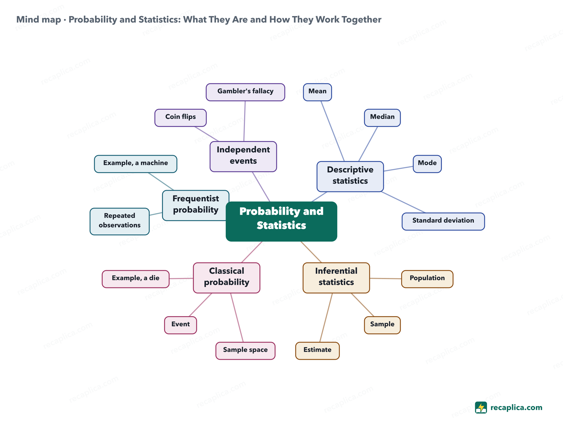
    Mind map: Probability and Statistics: What They Are and How They Work Together
    • Probability and Statistics
      • Descriptive statistics Summarizes data already collected
        • Mean
        • Median
        • Mode
        • Standard deviation
      • Inferential statistics Uses a sample to estimate a population
        • Population
        • Sample
        • Estimate
      • Classical probability Favorable outcomes over possible outcomes
        • Sample space
        • Event
        • Example, a die
      • Frequentist probability Observed frequency over many trials
        • Repeated observations
        • Example, a machine
      • Independent events One event doesn't change the odds of another
        • Coin flips
        • Gambler's fallacy

    Quiz: test yourself

    Answer the questions to check what you have learned: you get instant feedback and a short explanation.

    Grade 0/10 0/5
    1 What is the main difference between descriptive and inferential statistics?

    Descriptive statistics organizes and summarizes the data on hand; inferential statistics uses a sample to estimate characteristics of a larger population.

    2 How is the classical probability of an event calculated?

    Classical probability is the ratio between favorable outcomes and all possible outcomes, and it only applies when outcomes are equally likely, as with a die roll.

    3 After five heads in a row, the probability of tails on the next flip goes up.

    False: coin flips are independent events, so the probability of heads or tails stays at 1/2 regardless of earlier flips. Believing otherwise is the gambler's fallacy.

    4 Why does the median hold up better than the mean against outliers?

    The mean adds up every value and divides by their count, so one very high or very low number shifts it; the median only looks at the middle position of the ordered list, which stays put.

    5 What does the standard deviation of a data set measure?

    Standard deviation is small when data cluster close to the mean and large when they're more spread out: it measures how dispersed the values are around the mean.

    Answers: 1-A · 2-A · 3-B · 4-A · 5-A

    Flashcards

    Tap the card to flip it and check whether you remember the answer, then move to the next one.

    1 / 8

    Explain it in your own words

    The ultimate test: if you can explain it in simple words, you've truly understood it. Write your explanation, then compare it with the Recap.

    Your explanation is saved only on this device.

    Probability and statistics are two branches of mathematics that study uncertainty from opposite directions: probability calculates ahead of time how likely an event is to happen, while statistics analyzes data already collected, either to describe it or to draw conclusions about a wider group. Introductory math courses teach them together because they share the same basic tools, from the idea of an event to that of a sample. Statistics itself splits into descriptive statistics, which summarizes data with numbers like the mean and standard deviation, and inferential statistics, which uses a sample to estimate an entire population. Probability, in turn, is calculated differently depending on whether outcomes are equally likely (classical probability, like a die roll) or observed over time (frequentist probability, like equipment failures).

    Frequently asked questions

    What's the difference between probability and statistics?

    It comes down to timing: probability applies before an event happens, to work out how likely it is; statistics applies after, once data has already been gathered, to summarize it or to estimate a wider group from a sample. Introductory math courses teach them together because they share the same basic tools, such as the concept of an event and of a sample.

    What is descriptive and inferential statistics, together?

    It's the pairing of the two approaches within statistics: the descriptive side summarizes data with numbers like the mean and standard deviation, the inferential side uses a sample to estimate the values of a larger population when observing the whole group isn't possible.

    How do you calculate the mean of a group of numbers?

    You add up all the values and divide the result by how many values there are; for example, adding the ages of a group of students and dividing by the number of students gives the group's average age.

    What is the gambler's fallacy?

    It's the mistaken belief that after a run of identical results (for example five heads in a row on a coin), the opposite result becomes more likely on the next try. In reality, each flip is an independent event and the probability stays exactly the same.

    What is standard deviation used for?

    It shows how closely the data in a set cluster around the mean or how far apart they're spread: a small value means the data sit close to the mean, a large value means they're more scattered.

    Sources

    • OpenStax, Introductory Statistics 2e
    • Stanford Encyclopedia of Philosophy, Interpretations of Probability
    • Statistics LibreTexts, Gambler's Fallacy
    • ISTAT, Resident Population

    Every Recap goes through an independent review before publication.

    Every evening, the day's new Recaps on our Telegram channel. Join the channel →

    Keep learning

    • Science Cognitive Load Theory: The Definition Behind Sweller's Research Cognitive load is the amount of working memory a task uses up while you learn something new. Psychologist John Sweller first described it in 1988, starting from research on problem solving: a strategy that is too demanding leaves little room to build stable mental structures. Later research distinguishes three types of load, intrinsic, extraneous, and germane, though part of the field treats the third as indistinguishable from the first. Cutting extraneous load, with worked examples or less cluttered materials, frees up mental room for actual learning. Read the Recap →
    • Science Cognitivism: how the mind processes information Cognitivism is the psychological paradigm that treats the mind as a system for processing information, spanning perception, memory, reasoning and language. The shift began around 1956, while behaviorism, championed by Watson and Skinner, still ruled academic psychology and reduced the field to observable stimuli and responses. That same year, George Miller exposed the limits of short-term memory, and Chomsky joined McCarthy, Minsky, Newell and Simon in laying the groundwork for cognitive science. Donald Broadbent's attention model in 1958 and Ulric Neisser's 1967 book, which put the name cognitive psychology into common use, complete the roster of its founding figures. Read the Recap →
    • Science Behaviorism: What It Is and Where It Came From Behaviorism is the school of psychology that studies only observable behavior, leaving aside the thoughts and feelings that stay hidden inside the mind. It began in 1913, when the American psychologist John B. Watson published an essay calling for psychology to become an experimental science, without relying on introspection. After him, Ivan Pavlov studied conditioned reflexes and Edward Thorndike studied trial-and-error learning; Burrhus Skinner pushed the ideas to their most extreme form with radical behaviorism. The thread running through all of it is the stimulus-response model: a behavior is explained by what comes before it and what follows it, not by guessing what happens inside the head of the person doing it. Read the Recap →

    recaplica

    Clear in 30 seconds, yours in 10 minutes.

    Recaps Mind maps Request a Recap Telegram channel Mind map maker Our method About Privacy & cookies Legal notes & terms of use

    © 2026 Recaplica · A project by Curi S.r.l. — VAT IT05472000750

    Statistics, only if you say so

    To learn which Recaps help most we would use Google Analytics, with aggregate, anonymous data. It starts only with your OK, and you can change your mind anytime. Privacy policy