Skip to content
recaplica

    One moment: security check

    Cloudflare wants to make sure you're not a robot. Tick the box below and your search will continue on its own.

    IT
    recaplica First order differential equations: how to solve them
    © 2026 Recaplica · recaplica.com — All rights reserved
    Home › Science

    First order differential equations: how to solve them

    By Recaplica Newsroom · Updated on October 13, 2026

    What to print

    Page numbers appear when printing with default margins.

    Slides

    Choose a cut

    Flash10 slidesThe essential thread, to present in classFull15 slidesEvery chapter and the deeper detail

    Both come with speaker notes.

    Telegram channel
    recaplica Clear in 30 seconds, yours in 10 minutes.
    In 30 seconds Key points Deep dive Slides Myths Mind map Quiz Flashcards FAQ

    In 30 seconds quick read

    A first order equation ties an unknown function to its first derivative, and the method you reach for depends on the form you can rewrite it in. If all the y terms can be separated from all the x terms, the equation is separable, so you separate and integrate. Rewrite it as y' + p(t)y = g(t) and it is linear, so you multiply through by the integrating factor. If the right-hand side depends only on the ratio y/x it is homogeneous, and the substitution v = y/x sends you back to the separable case. The initial condition comes in at the very end, to pin down the constant.

    Key Points

    • A first order differential equation involves the first derivative of the unknown function and no higher ones.
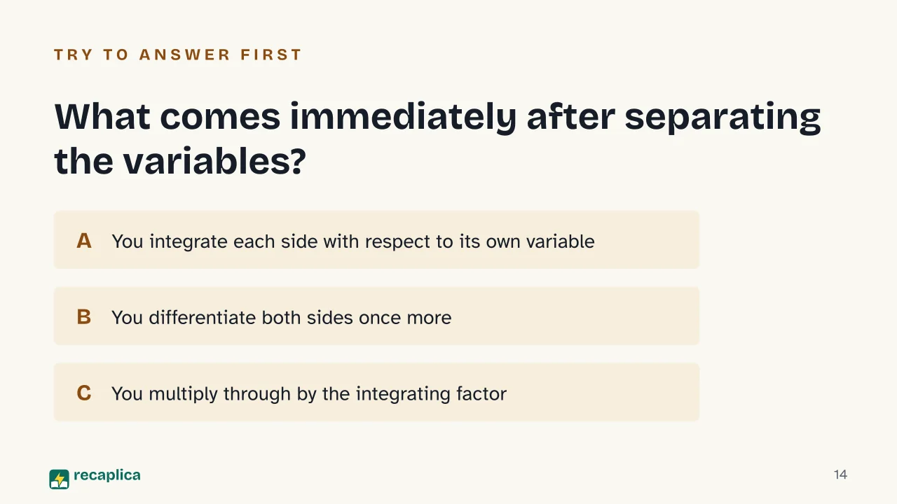
    • Separation of variables takes two moves, separating the sides and then integrating each one with respect to its own variable.
    • Values of y that make the y factor vanish give constant solutions, which have to be checked on their own because separating can lose them.
    • The integrating factor is the exponential of the integral of p, and it makes the derivative side integrable in a single step.
    • Setting v = y/x turns a homogeneous equation into a separable one in the variables v and x.
    • For a linear equation, p and g being continuous on an interval is enough to guarantee one single solution of the initial value problem there.

    Deep Dive

    Three shapes to spot first

    A first order differential equation relates an unknown function and its first derivative. How you solve it depends on the form you manage to rewrite it in, and three structures keep coming back in introductory courses: the separable equation, the linear one and the homogeneous one. Recognising the structure comes before any calculation, because each one has a procedure of its own. For the general definition of a differential equation and the wider picture, there is the Recap on what differential equations are and how they work.

    Separable equations

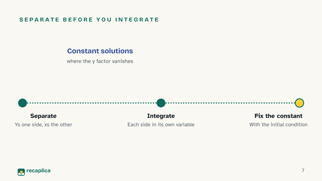
    According to Paul’s Online Math Notes, an equation is separable when it can be rewritten with all the y terms, multiplied by the derivative, on one side and all the x terms on the other. The procedure then takes two moves: you separate the variables, and you integrate each side with respect to the variable that belongs to it. The integrals are the ones from calculus, and the integration is where an arbitrary constant comes from. OpenStax flags one further check: where the y factor vanishes, constant solutions appear, and they have to be examined on their own. Wolfram MathWorld gives the reason behind that check — the separation step divides by that factor, and dividing can drop exactly those solutions along the way.

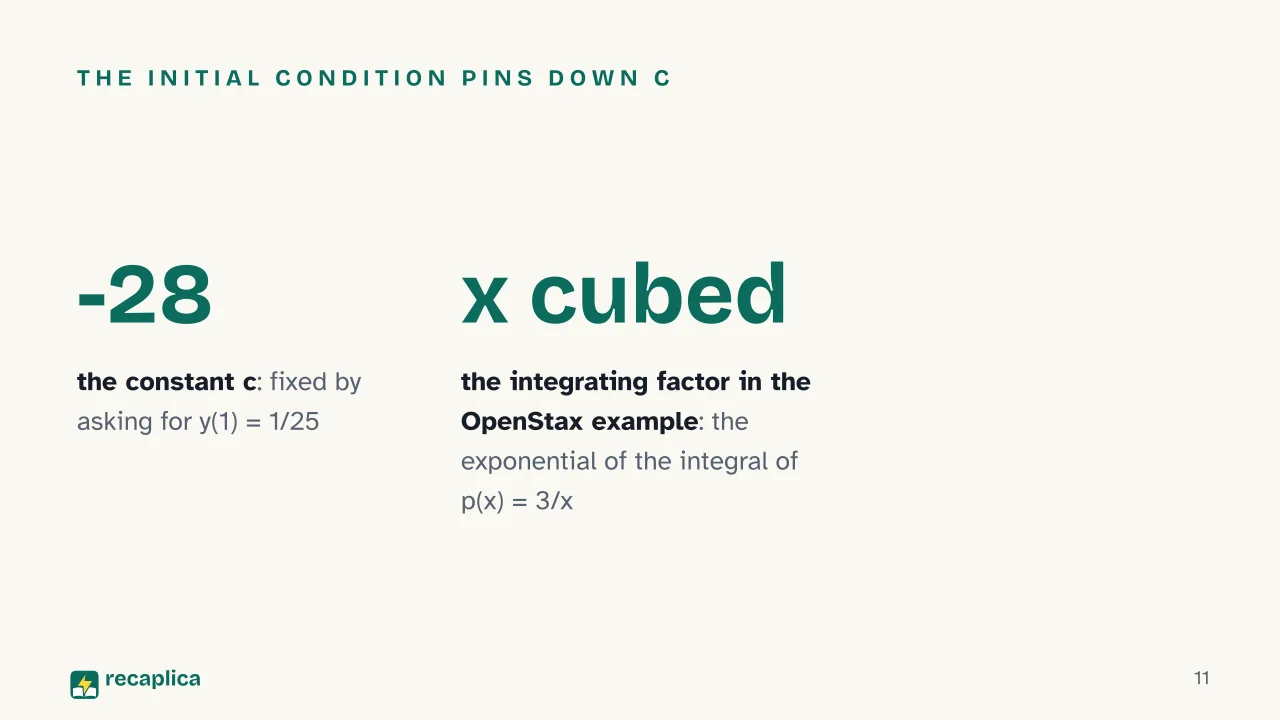
    Practical example: Paul’s Online Math Notes works through the initial value problem y′ = 6y²x with the condition y(1) = 1/25. Separating the variables and integrating gives the implicit solution −1/y = 3x² + c. The initial condition fixes the constant at c = −28, and the explicit solution becomes y(x) = 1/(28 − 3x²). That function holds for −√(28/3) < x < √(28/3), because the denominator vanishes at the ends of the interval.

    That last step is part of the answer. The solution of an initial value problem arrives together with the interval it exists on, and the formula means something only inside it.

    OpenStax adds a second case, y′ = (x² − 4)(3y + 2), which under the same method gives the general solution y = (−2 + c·e^(x³−12x))/3, with c an arbitrary constant. The plane where you read off those solution curves has its own Recap in analytic geometry.

    Linear equations and the integrating factor

    The standard form of a first order linear equation is y′ + p(t)y = g(t), with p and g continuous functions. OpenStax starts from an equivalent way of writing it, a(x)y′ + b(x)y = c(x), which turns into the standard one once you divide by a(x). At that point an auxiliary function comes in, the integrating factor µ: multiply both sides by µ and the derivative side becomes integrable in a single step. The factor comes out as the exponential of the integral of p, and the constant that integral brings along can be taken equal to 1. Anyone who wants to revisit linear equations in the algebraic sense can start from linear algebra.

    Practical example: OpenStax applies the method to x·y′ + 3y = 4x² − 3x for x > 0. Dividing by x gives the standard form, with p(x) = 3/x and q(x) = 4x − 3, and the integrating factor computed for this equation is µ(x) = x³. Multiplying both sides by x³ and integrating leads to the general solution y = 4x²/5 − 3x/4 + c/x³. If the problem comes with an initial condition, the last step uses it to fix c.

    The method extends beyond textbook exercises. Paul Dawkins applies it to a falling-body model with air resistance, where the integrating factor leads to the general solution v = 50 + c·e^(−0.196t), later fixed by the initial velocity.

    Homogeneous equations and the substitution v = y/x

    A first order equation is called homogeneous when it can be written as y′ = F(y/x), that is, when the right-hand side depends only on the ratio between y and x. Here you change variable: setting v = y/x makes the equation separable in the variables v and x, and you are back in the procedure above. Once the equation in v is solved, you put y/x back in place of v to recover the function you were after. Wolfram MathWorld records the same definition and confirms that the change of variable leads to a closed-form solution; in the example with an initial condition worked through by Paul Dawkins, once v goes back to y, the solution comes out explicit, and the initial condition decides which sign of the square root to keep.

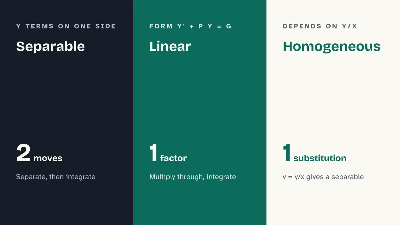
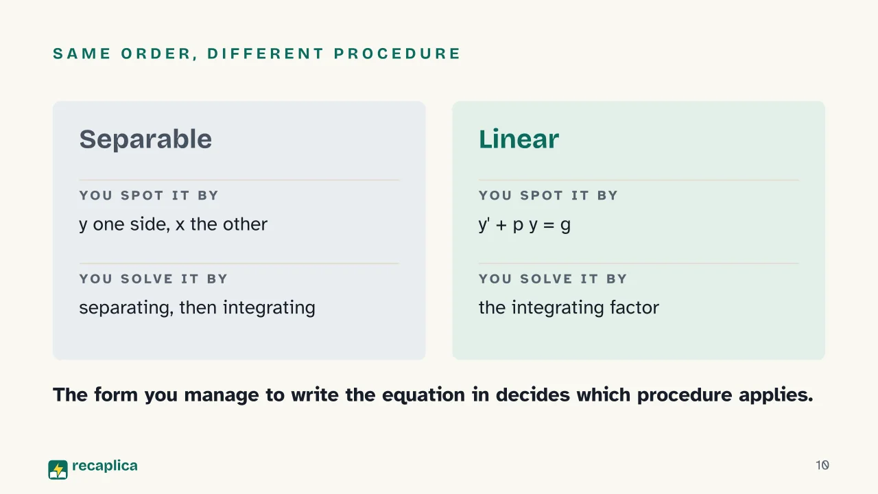
    FormHow to spot itSolving move
    Separabley terms with the derivative on one side, x terms on the otherseparate, then integrate both sides
    Linearit rewrites as y′ + p(t)y = g(t)multiply by the integrating factor µ(t)
    Homogeneousthe right-hand side depends only on y/xsubstitute v = y/x and solve the separable

    How many solutions an initial value problem has

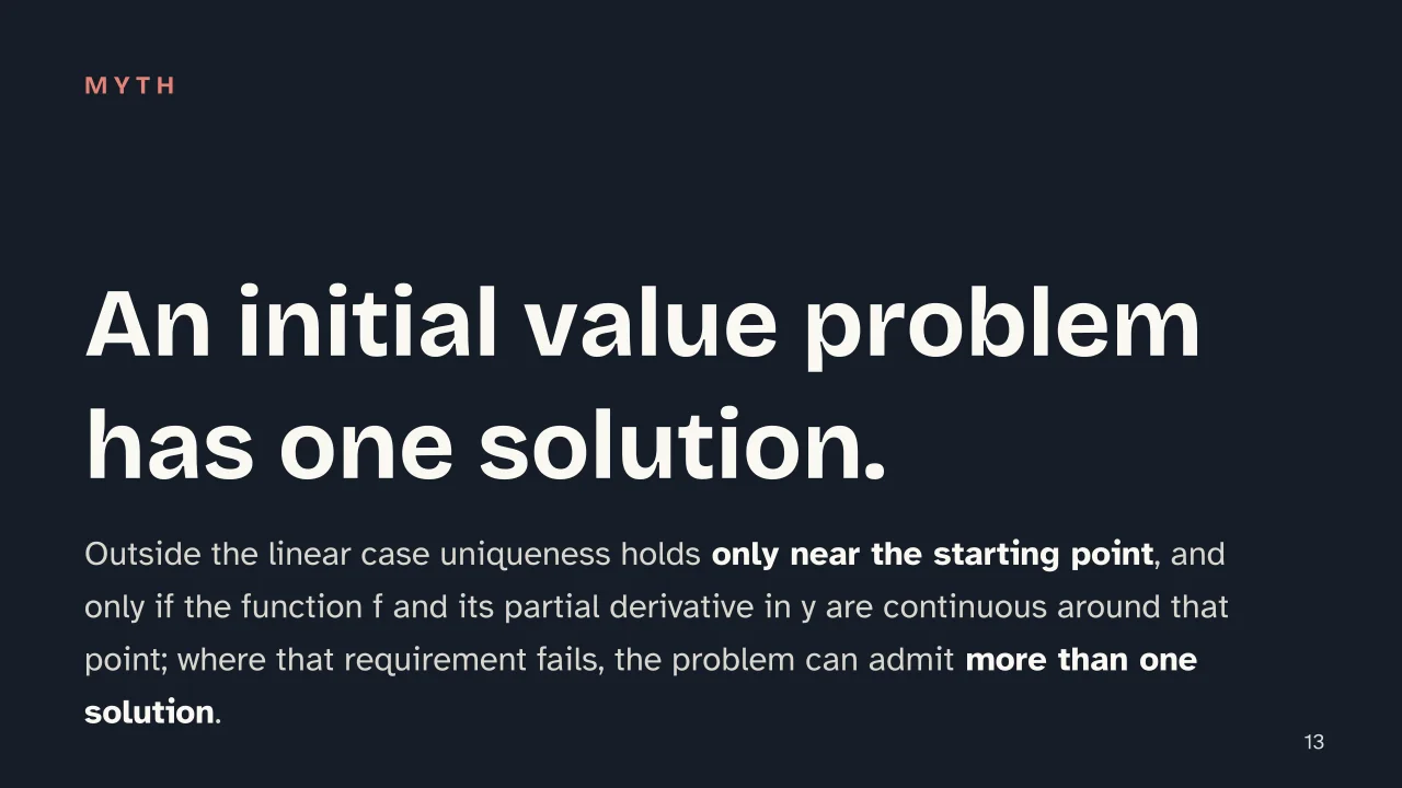
    For linear equations the answer is clean: if p(t) and g(t) are continuous on an interval, the problem with an initial condition has one and only one solution on that interval. Step outside the linear case and the guarantee weakens. Uniqueness holds only locally, on an interval that may be small, and on condition that the function f and its partial derivative with respect to y be continuous near the starting point. MIT OpenCourseWare presents this existence and uniqueness theorem as a central technical result in the theory of differential equations, and points to its standard proof, Picard iteration, which builds the solution by successive approximations.

    When those hypotheses fail, there can be more than one solution. Paul’s Online Math Notes works through a problem where the derivative of f with respect to y is discontinuous at y = 0 and which accepts both y = 0 and y(t) = ±(2t/3)^(3/2).

    Slide deck

    Slides ready to download and make your own in PowerPoint or Google Slides, with speaker notes. Pick the Flash cut or the Full one.
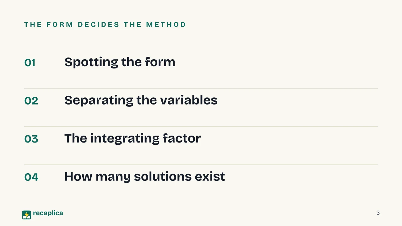
    Slide 1 of the presentation on First order differential equations: First order equationsSlide 2 of the presentation on First order differential equations: What form is this equation in?Slide 3 of the presentation on First order differential equations: The form decides the methodSlide 4 of the presentation on First order differential equations: Chapter 01: Spotting the formSlide 5 of the presentation on First order differential equations: Separable · Linear · HomogeneousSlide 6 of the presentation on First order differential equations: Chapter 02: Separating the variablesSlide 7 of the presentation on First order differential equations: Separate before you integrateSlide 8 of the presentation on First order differential equations: Where does that formula still hold?Slide 9 of the presentation on First order differential equations: Chapter 03: The integrating factorSlide 10 of the presentation on First order differential equations: Same order, different procedureSlide 11 of the presentation on First order differential equations: The initial condition pins down cSlide 12 of the presentation on First order differential equations: Chapter 04: How many solutions existSlide 13 of the presentation on First order differential equations: An initial value problem has one solution.Slide 14 of the presentation on First order differential equations: What comes immediately after separating the variables?Slide 15 of the presentation on First order differential equations: Now go over it again
    Flash10 slidesThe essential thread, to present in classFull15 slidesEvery chapter and the deeper detail

    Common myths

    • ✗ Myth An initial value problem always has exactly one solution.

      ✓ Reality In the linear case that holds as soon as p and g are continuous. Outside it, uniqueness requires that f and its partial derivative in y remain continuous near the starting point, and where that fails the problem can admit more than one solution: Paul's Online Math Notes works through an example that accepts both y = 0 and y(t) = ±(2t/3)^(3/2).

    • ✗ Myth Separation of variables works on any first order equation.

      ✓ Reality Separating works only when the ys and the xs can be pulled onto opposite sides of the equals sign. A linear equation in standard form usually resists, and the integrating factor handles it instead; a homogeneous equation goes through the substitution v = y/x first, which makes it separable in the new variables.

    • ✗ Myth Once you have the formula for the solution, the exercise is finished.

      ✓ Reality You still owe an answer about where that formula works. In the problem solved in Paul's Online Math Notes the solution y(x) = 1/(28 − 3x²) makes sense for −√(28/3) < x < √(28/3), because the denominator hits zero at the ends of that stretch.

    Mind map

    Drag the background to move around and the nodes to reposition them; use − and + to collapse and expand branches.
    Customize
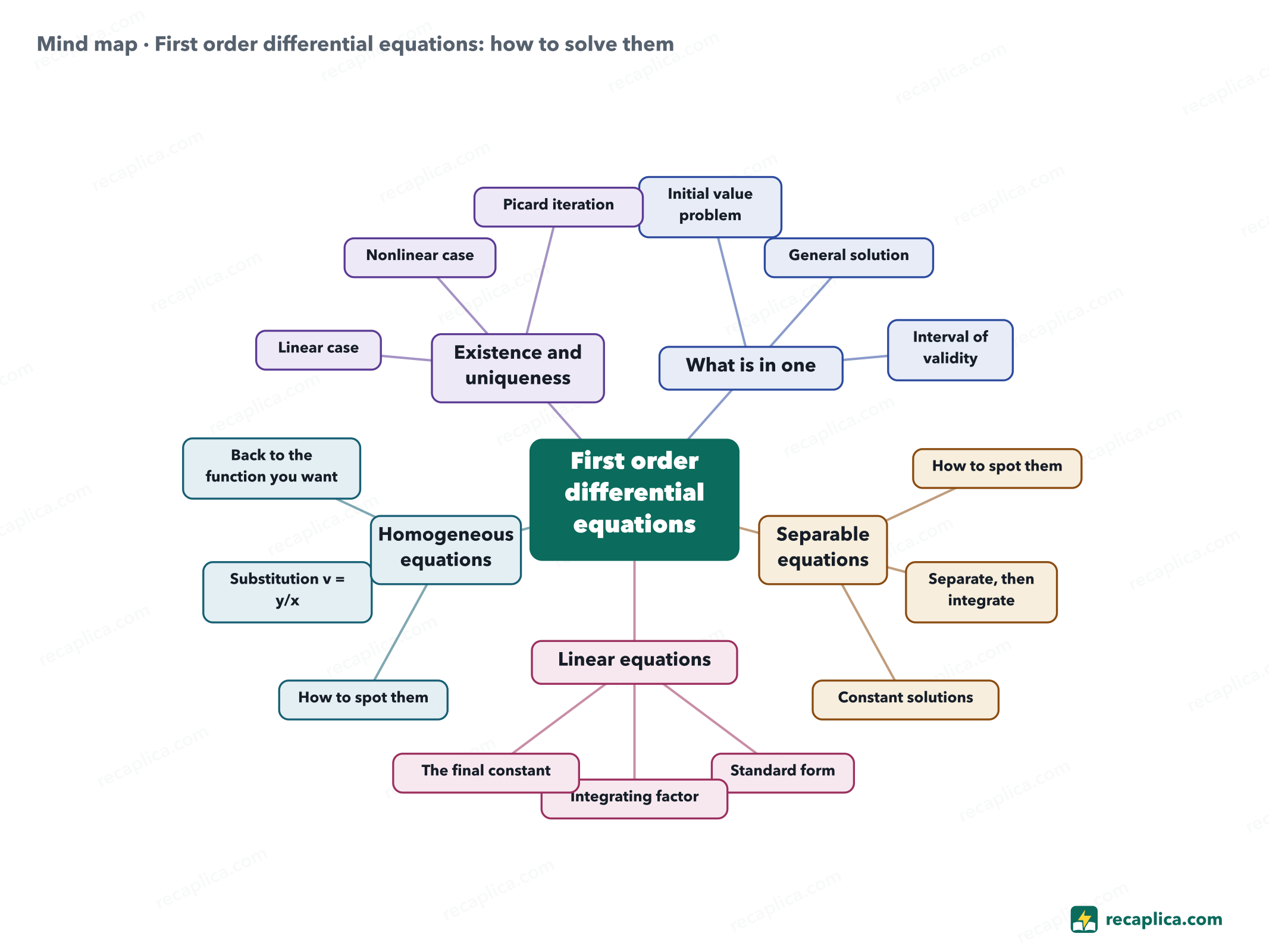
    Mind map: First order differential equations: how to solve them
    • First order differential equations
      • What is in one The unknown function and its first derivative
        • Initial value problem The equation plus one initial condition
        • General solution It carries an arbitrary constant
        • Interval of validity
      • Separable equations
        • How to spot them The y terms on one side, the x terms on the other
        • Separate, then integrate
        • Constant solutions Where the y factor vanishes
      • Linear equations
        • Standard form y' + p(t)y = g(t), with both functions continuous
        • Integrating factor The exponential of the integral of p
        • The final constant The initial condition fixes it
      • Homogeneous equations
        • How to spot them The right-hand side depends only on y/x
        • Substitution v = y/x It leads to a separable equation
        • Back to the function you want Put y/x back in place of v
      • Existence and uniqueness
        • Linear case p and g continuous on an interval is enough
        • Nonlinear case The partial derivative in y has to be continuous too
        • Picard iteration It builds the solution by successive approximations

    Quiz: test yourself

    Answer the questions to check what you have learned: you get instant feedback and a short explanation.

    Grade 0/10 0/5
    1 When is a first order equation called separable?

    That is the definition used in Paul's Online Math Notes, and what counts is how the y terms and the x terms can be arranged on the two sides.

    2 What comes immediately after separating the variables?

    First the two sides come apart, then each one gets integrated in the variable that belongs to it.

    3 In the problem y' = 6y²x with y(1) = 1/25, what is the constant c in the implicit solution -1/y = 3x² + c?

    Substituting the initial condition into the implicit solution gives c = -28, and from there the explicit solution y(x) = 1/(28 - 3x²).

    4 How do you obtain the integrating factor of a linear equation in standard form?

    You integrate p and then exponentiate, and whatever additive constant turns up there can be set to 1, since any function that makes the derivative side integrable will do.

    5 For a nonlinear equation, what guarantees a single solution near the starting point?

    With those two continuity requirements the initial value problem has a unique solution, defined at least on a small interval around the starting point.

    Answers: 1-C · 2-A · 3-B · 4-D · 5-A

    Flashcards

    Tap the card to flip it and check whether you remember the answer, then move to the next one.

    1 / 7

    Explain it in your own words

    The ultimate test: if you can explain it in simple words, you've truly understood it. Write your explanation, then compare it with the Recap.

    Your explanation is saved only on this device.

    A first order equation ties an unknown function to its first derivative, and the method you reach for depends on the form you can rewrite it in. If all the y terms can be separated from all the x terms, the equation is separable, so you separate and integrate. Rewrite it as y' + p(t)y = g(t) and it is linear, so you multiply through by the integrating factor. If the right-hand side depends only on the ratio y/x it is homogeneous, and the substitution v = y/x sends you back to the separable case. The initial condition comes in at the very end, to pin down the constant.

    Frequently asked questions

    What is the difference between a general solution and the solution of an initial value problem?

    A general solution carries an arbitrary constant along with it, left over from the integration. An initial value problem adds one initial condition, and that condition gives the constant a definite value: in the problem solved in Paul's Online Math Notes, asking for y(1) = 1/25 leads to c = -28.

    How do you tell which method to use?

    Look at the form the equation can be written in. Y terms on one side and x terms on the other means separable; the form y' + p(t)y = g(t) means linear, so integrating factor; a right-hand side that depends only on y/x means homogeneous, so the substitution v = y/x.

    Why does the solution hold only on a certain interval?

    Because the function you end up with can stop being defined. In the initial value problem solved by Paul Dawkins the denominator of the explicit solution vanishes at the ends of the stretch, and past those two points the formula means nothing.

    Do homogeneous equations need a method of their own?

    The change of variable v = y/x exists precisely to bring one back to a separable equation in the variables v and x. From there you integrate as you would in any separable case, then y/x goes back in place of v and you have the function you were after.

    Sources

    • Paul's Online Math Notes, Differential Equations, chapter 2 (Lamar University)
    • OpenStax, Calculus Volume 2, Separable Equations
    • OpenStax, Calculus Volume 2, First-order Linear Equations
    • Wolfram MathWorld, Separable Differential Equation
    • Wolfram MathWorld, Homogeneous Ordinary Differential Equation
    • MIT OpenCourseWare, ES.1803 Differential Equations, Existence and Uniqueness Theorem

    Every Recap goes through an independent review before publication.

    Every evening, the day's new Recaps on our Telegram channel. Join the channel →

    Keep learning

    • Science Correlation: What It Means and How to Read the Coefficient Correlation measures how closely two variables move together, and the most common way to put a number on it is the correlation coefficient, which runs from -1 to +1. A value near +1 means the two variables rise together, near -1 means one rises while the other falls, and near 0 means no linear relationship stands out. The coefficient only captures the strength of a straight-line relationship, and a single unusual data point can push it up or down by a lot. Even when it's strong, a correlation between two variables never shows that one causes the other. Read the Recap →
    • Science Light Refraction: What It Is, the Laws Behind It, and Examples A surface that separates two transparent materials sends some light back, reflecting it, and lets the rest through while bending it toward a new direction. The law of reflection keeps the incoming and outgoing angles equal, both measured from the normal to the surface. Snell's law governs refraction instead, linking the index of each material to how much the ray tilts before and after it crosses over. These two laws alone explain mirrors, lenses, prisms and everyday sights such as a pencil that appears to snap inside a glass of water. Read the Recap →
    • Science Total Internal Reflection and the Critical Angle: Definition and Formula Total internal reflection is what happens when a light ray stops being able to leave a transparent medium and gets sent back inside it completely. It takes place past a specific angle of incidence, called the critical angle, calculated with Snell's law by comparing the refractive indices of the two materials involved. It only happens under one precise condition: the ray must be traveling from an optically denser medium into a less dense one, such as from water into air or from glass into air. Optical fibers and, in part, the sparkle of diamonds rely on this same principle. Read the Recap →

    recaplica

    Clear in 30 seconds, yours in 10 minutes.

    Recaps Mind maps Request a Recap Telegram channel Mind map maker Our method About Privacy & cookies Legal notes & terms of use

    © 2026 Recaplica · A project by Curi S.r.l. — VAT IT05472000750

    Statistics, only if you say so

    To learn which Recaps help most we would use Google Analytics, with aggregate, anonymous data. It starts only with your OK, and you can change your mind anytime. Privacy policy