|
recaplica
Chi-Square Test: Formula, Example and Degrees of Freedom | |||||||||||||||||||||||||||||||||||||||||||||||||||||||||||||||||||||||||||||||||
| © 2026 Recaplica · recaplica.com — All rights reserved | |||||||||||||||||||||||||||||||||||||||||||||||||||||||||||||||||||||||||||||||||
Chi-Square Test: Formula, Example and Degrees of FreedomWhat to print Page numbers appear when printing with default margins. SlidesChoose a cut Flash10 slidesThe essential thread, to present in classFull15 slidesEvery chapter and the deeper detailBoth come with speaker notes. In 30 seconds quick readThe chi-square test compares the counts recorded in a table with the counts you would expect if a starting hypothesis were true. For each cell you take the gap between observed and expected, square it and divide by the expected count, then add up all the cells. If the total is larger than a critical value, which depends on the degrees of freedom, the hypothesis is rejected. The test tells you whether two classifications are related, and it can also check whether data follow a predicted distribution. When expected counts are very small, the result can no longer be trusted. Key Points
Key figures
Deep DiveThe chi-square test (written χ², and also called the chi-squared test) is a test on counts: how many times each category turns up in a sample. It sets those counts, the observed frequencies, against the ones you should see if a starting hypothesis were true, the expected frequencies. Karl Pearson published it in 1900. MacTutor, the history of mathematics archive at the University of St Andrews, says Pearson’s aim with the test was to end the normal distribution’s central role. One calculation answers two questions. A test of independence asks whether two ways of classifying the same items are related; a goodness of fit test asks whether a sample behaves the way a chosen distribution predicts. Null and alternative hypotheses in a chi-square testChi-square is a good place to see how probability and statistics work together: a number computed from the data is checked against a probability distribution to choose between two hypotheses. The first, the null hypothesis H₀, is the one the calculation puts on trial. In a test of independence, the NIST handbook of statistical methods states the null hypothesis as the two classifications being independent. Put another way, the chance of landing in a given cell equals the chance of its row multiplied by the chance of its column, the same multiplication rule used for independent events when you calculate probability. The alternative hypothesis claims the product fails in at least one cell, which would mean the classifications depend on each other. For goodness of fit, H₀ says the data follow the stated distribution and the alternative says they depart from it. The chi-square test formulaFor every cell, take the observed frequency O and the expected frequency E, square the difference and divide by E. The statistic is the sum of all those pieces: χ² = Σ (O − E)² / E In a test of independence the expected counts come from the table’s totals. For a single cell: E = (row total × column total) / grand total A large statistic means the observed counts sit far from the expected ones. Yale’s statistics course reads this, for goodness of fit, as a sign that the proposed model describes the data badly. When the null hypothesis holds, the value roughly follows a chi-square distribution, which NIST defines as the sum of the squares of ν independent standard normal variables, ν being the degrees of freedom. Chi-square test example: wafer defects across three shiftsNIST, the US federal standards agency, works through a factory case. A plant records 309 defects on wafers, sorted by type (A, B, C, D) and by production shift (1, 2, 3), and wants to know whether the mix of defects changes from one shift to the next. The two classifications make a contingency table with 3 rows and 4 columns; expected frequencies are in brackets.
Repeat that for all twelve cells and add them up, and NIST arrives at χ² = 19.18. The table has (3 − 1)(4 − 1) = 6 degrees of freedom, and at a 0.05 significance level the critical value for 6 degrees is 12.5916. Since 19.18 is higher, the independence hypothesis is rejected: in NIST’s reading, the data give significant evidence that the share of each defect type changes with the shift. The example’s p-value is 0.00387. Degrees of freedom in the chi-square testDegrees of freedom count how many cells can still vary once the totals are fixed. In a goodness of fit test with k categories there are k − 1. Yale’s course points out that the last count has no room to move, because the counts have to add up to the total. Each parameter estimated from the data costs one more, so with d estimated parameters you end up at k − 1 − d. NIST writes the same rule as k − c, with k counting the classes that are not empty and c equal to the estimated parameters plus one. In its normality example two parameters are estimated, so c is 3. For a contingency table, (r − 1)(c − 1), where c now stands for columns, follows from the same reasoning. There are r·c cells, and after the constraint on the grand total rc − 1 of them are free; subtract the (r − 1) + (c − 1) parameters estimated for the row and column totals and exactly (r − 1)(c − 1) remain. Chi-square goodness of fit test: the pea seed exampleGeneticists use the goodness of fit version to check whether counts match an expected ratio. Phillip McClean’s genetics course at North Dakota State University takes a set of pea seeds whose predicted ratio is 9:3:3:1, and counts 556 of them.
Each expected count is the ratio’s fraction applied to the total, so 9/16 of 556 gives 312.75. Four classes mean 3 degrees of freedom, and the statistic comes to 0.47. At 3 degrees of freedom the table puts the 0.05 critical value at 7.82 (7.815 in the NIST table), and 0.47 corresponds to a probability above 0.90. The page concludes that the data are consistent with the 9:3:3:1 ratio. NIST adds two cautions for this use. The test needs data grouped into classes, so loose observations first have to go into frequency tables for categorical variables, and the value of the statistic depends on how those classes are drawn. Discrete distributions, the binomial and the Poisson among them, can be tested this way too. Chi-square independence test vs goodness of fit test
How to read the resultPearson’s chi-square test looks at one tail only, the upper one. You find the column for 1 − α in the table and reject the null hypothesis when the statistic is larger than the value listed there. A few thresholds from the NIST table:
McClean’s page treats 0.05 as the conventional threshold. A significant result tells you an association is there. Bewick, Cheek and Ball, who wrote a review of tests of association in Critical Care in 2004, caution that the test by itself does not say how strong it is. To find the cells that matter most, look at the standardized residuals, which are built on the gap between observed and expected; any beyond 2 in absolute value are significant.
When the chi-square test is the wrong choiceThe chi-square distribution is an approximation, and it only works when expected counts are big enough. NIST says the approximation needs a large enough sample to be valid. Bewick and colleagues put a number on it, with the rule they attribute to Cochran: no cell may have an expected count under 1, and at most 20% of cells may fall under 5. Their way out is to combine categories where that makes sense. For 2×2 tables with few cases, the options are Yates’s continuity correction and Fisher’s exact test. Yates’s correction raises the smallest frequency by 0.5 and adjusts the others so the totals stay unchanged.
In large samples chi-square, Fisher and Yates land close together; in small ones Fisher and Yates return higher, more cautious P values. There is no full agreement on which to prefer; Bewick and colleagues report that Bland recommends Fisher or Yates for a more conservative approach. Paired data are a separate case, for instance the same patients measured twice. Chi-square ignores the pairing, so these tables go to McNemar’s test. Slide deckSlides ready to download and make your own in PowerPoint or Google Slides, with speaker notes. Pick the Flash cut or the Full one.     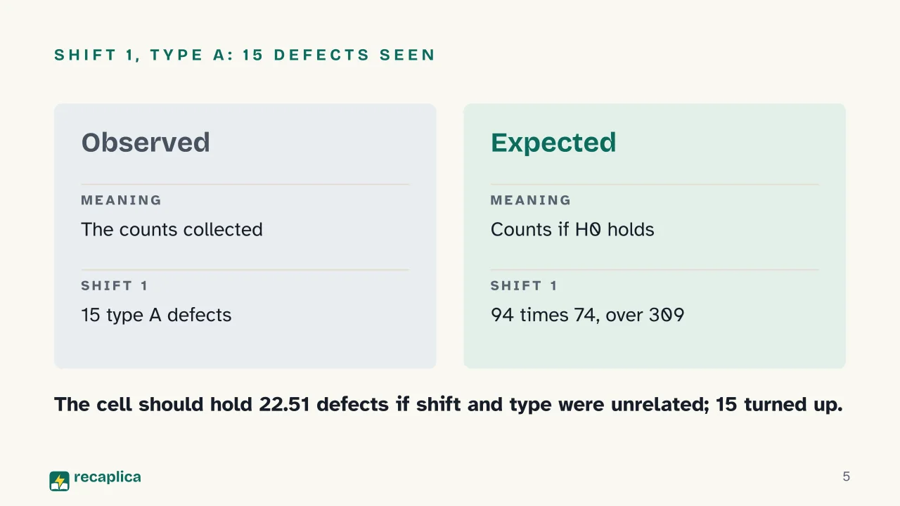  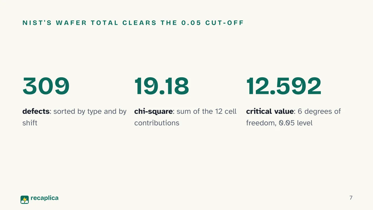  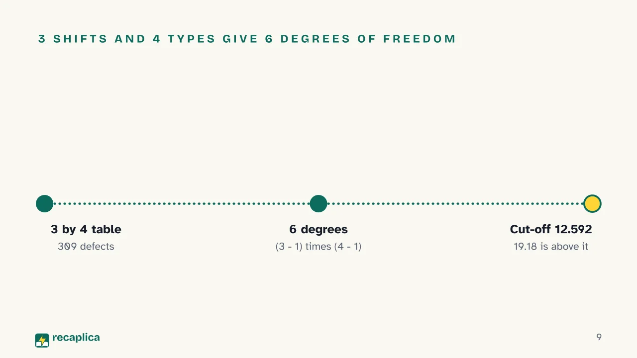 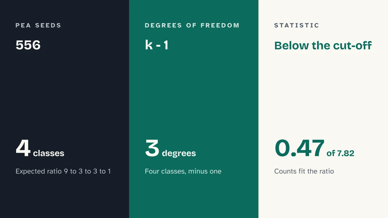  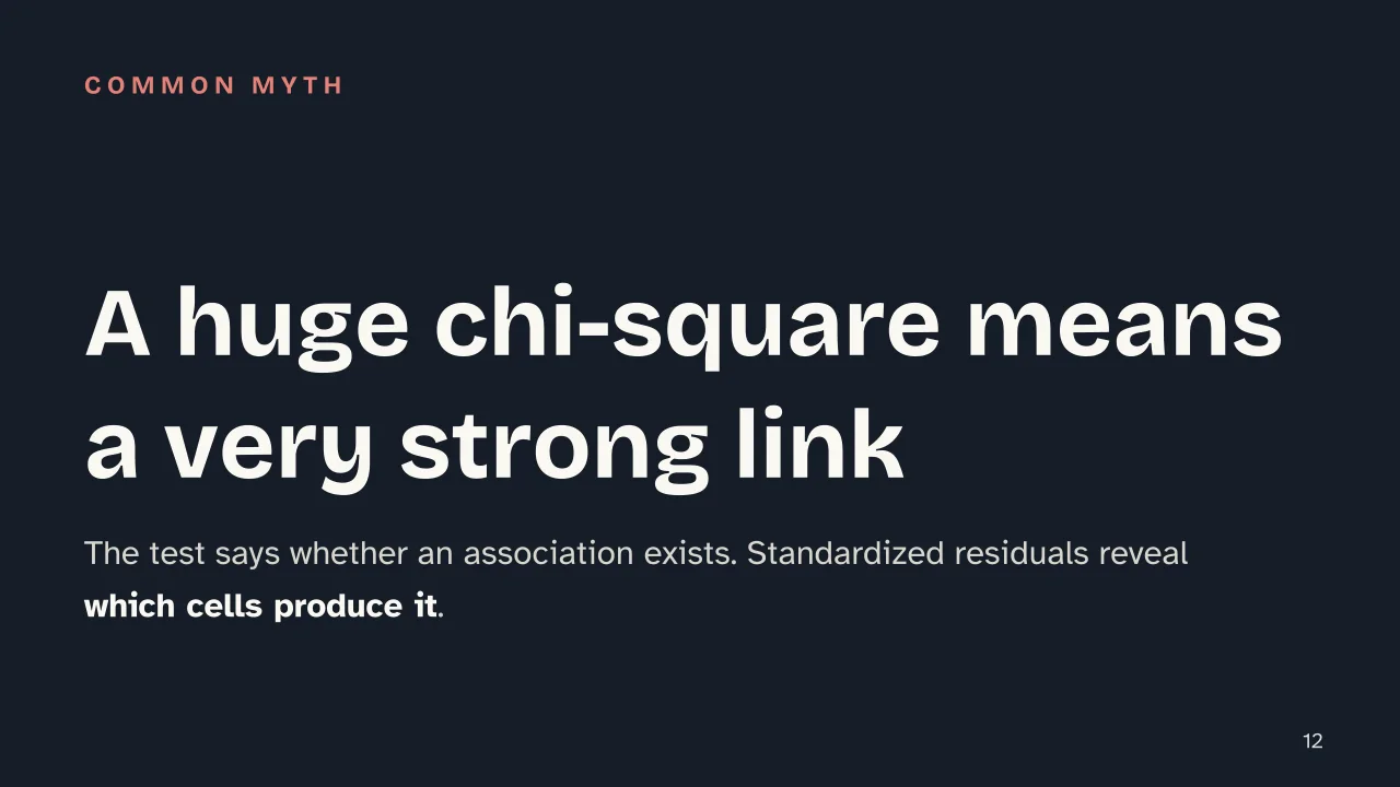 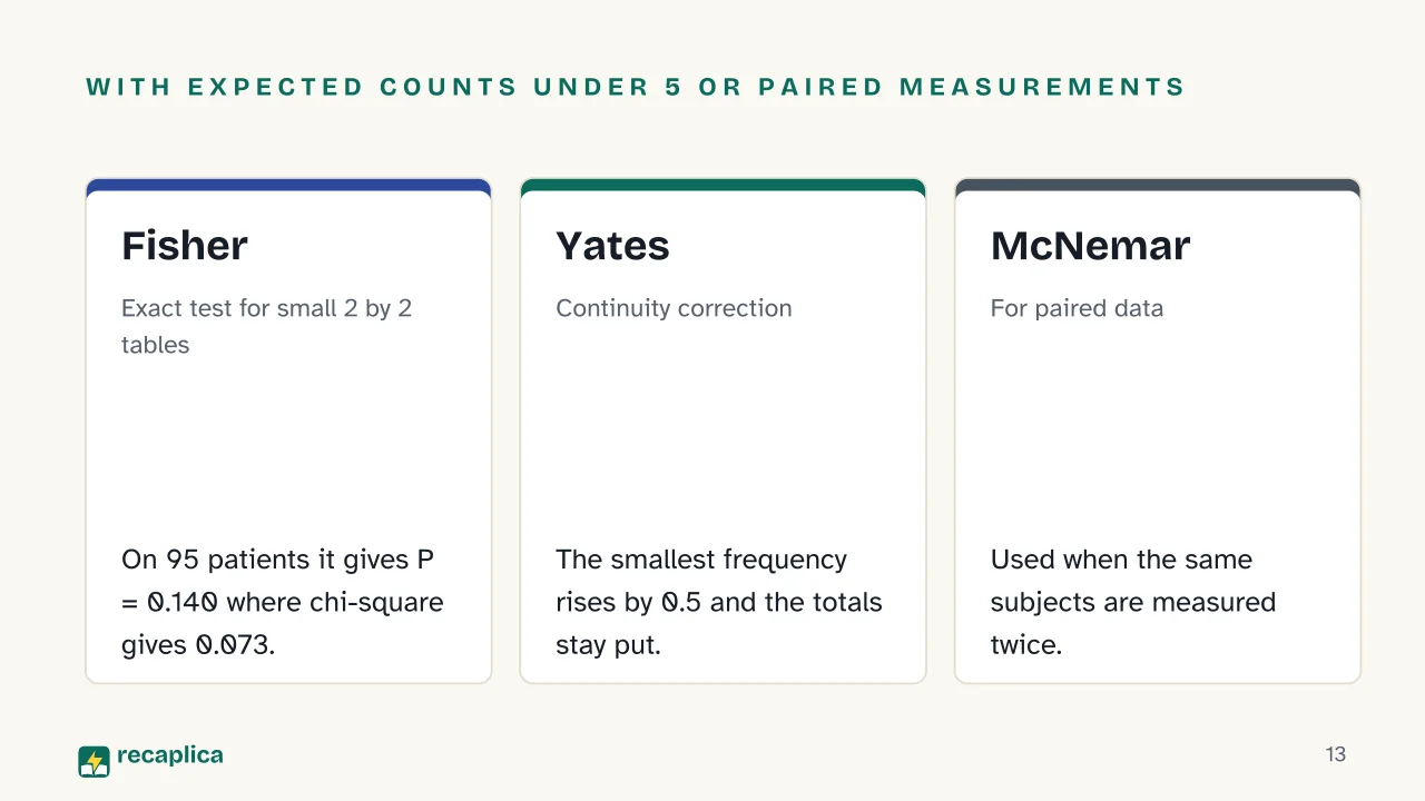 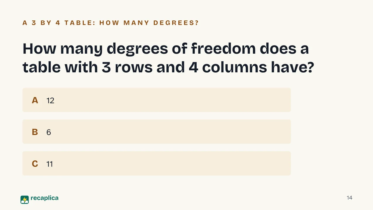  Common myths
Mind mapDrag the background to move around and the nodes to reposition them; use − and + to collapse and expand branches. 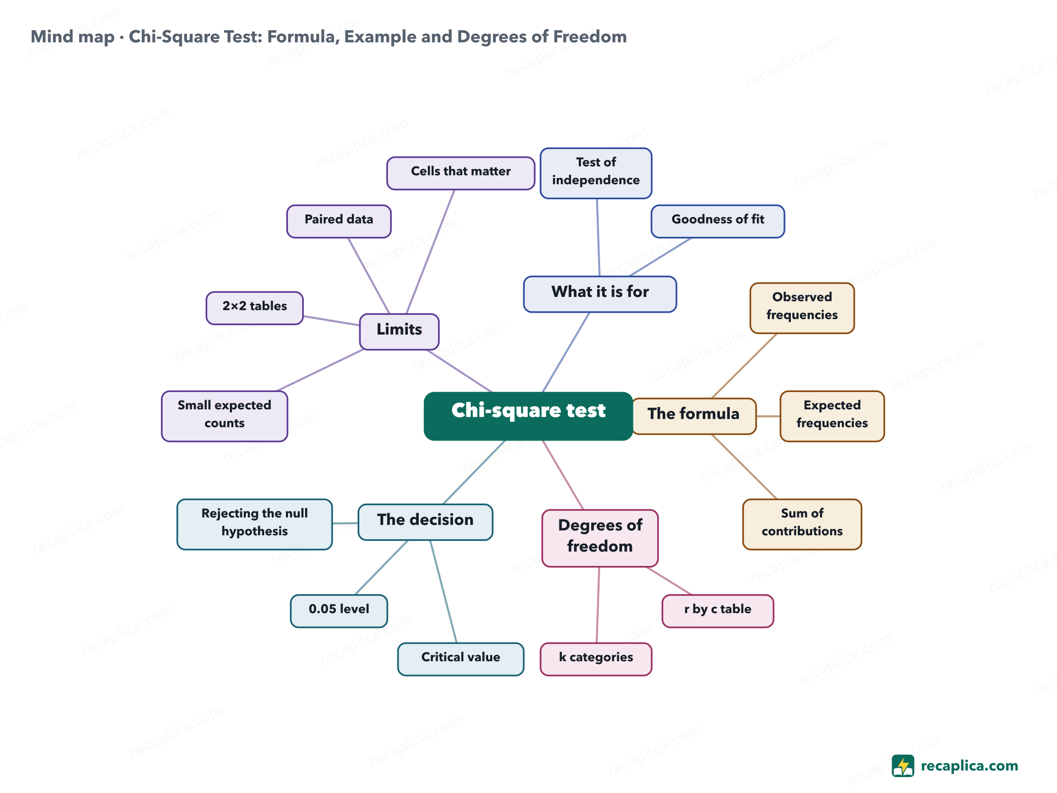
Quiz: test yourselfAnswer the questions to check what you have learned: you get instant feedback and a short explanation. Grade 0/10 0/5
FlashcardsTap the card to flip it and check whether you remember the answer, then move to the next one. 1 / 7 Explain it in your own wordsThe ultimate test: if you can explain it in simple words, you've truly understood it. Write your explanation, then compare it with the Recap. Your explanation is saved only on this device.
Frequently asked questionsWhat is the chi-square test formula and how do you calculate it?Start from the table of observed counts and work out the expected ones; in a contingency table each expected count is the row total times the column total, divided by the grand total. Then compute (O − E)² / E for every cell and add the results. Compare the sum with the critical value in the table for the right number of degrees of freedom. How many degrees of freedom does a chi-square test have?It depends on the test. For a table with r rows and c columns the answer is (r − 1)(c − 1), so a 3×4 table has 6. For goodness of fit, count the categories and subtract one; every parameter you had to estimate takes away another. What is the difference between a chi-square independence test and a goodness of fit test?The independence test takes two classifications of the same items, such as defect type and work shift, and checks whether they are related. Goodness of fit works with a single classification and asks whether the counts match a distribution or ratio set in advance, like the 9:3:3:1 ratio of the pea seeds. Both use the same formula; expected counts and degrees of freedom are worked out differently. When should you not use a chi-square test?When expected counts are too small (by the rule attributed to Cochran, none under 1 and no more than 20% under 5) and when the data are paired. In the first case you can merge categories or, for 2×2 tables, switch to Fisher's exact test or Yates's correction. In the second, McNemar's test is the one to use. What does a significant chi-square result mean?The statistic has passed the critical value at the chosen level, usually 0.05, so the null hypothesis is rejected. In a test of independence this signals an association between the two variables. Standardized residuals show which cells produce it. Every Recap goes through an independent review before publication. |